
As part of the Commerce Data Usability Project, Earth Genome in collaboration with the Commerce Data Service has created a tutorial that will guide you though processing and visualizating Digital Elevation Model (DEM) data. If you have question, feel free to reach out to the Commerce Data Service at DataUsability@doc.gov or Earth Genome at Dan@earthgenome.org.
The Dow Chemical facility in Freeport, Texas is the largest chemical manufacturing complex in the Western Hemisphere.
The site produces billions of dollars of product each year and employs thousands of people. To do this, the complex requires a lot of fresh water, drawing 100,000 gallons per minute from the Brazos River. This is a challenge when the Brazos River is plagued by drought, punctuated by flood conditions. The variability is not good for business. Dow has a strong, business incentive to encourage development of more sustainable and resilient freshwater supply from the Brazos River Basin. The river basin covers 45,000 square miles, whereas the footprint of the Freeport facility is eleven square miles. Dow cannot solve this problem alone and actively engages with upstream farmers, cities, industry, and local water authorities. The problem, however, is that finding a practical solution requires an understanding of a wide range of variables and interests, which must be expressed in common terms. The value and price of water can be highly divergent; the risk and return to water infrastructure investments are not always understood; and nature-based solutions are relatively new. There are just too many unknowns to even consider "green" infrastructure, or natural based solutions to water supply problems. All this makes a sound economic assessment of integrated, natural infrastructure projects very difficult, and until now, prohibitively expensive.
Enter GIST, the Green Infrastructure Support Tool. The web-based tool was created by the Earth Genome, a 501(c)(3) nonprofit organization, in collaboration with Arizona State University, Dow, and the World Business Council for Sustainable Development to identify and evaluate wetland restoration opportunities to support a more predictable and sustainable water supply to the Freeport facility. Wetlands store water during deluge and release water during dry spells, much like engineered solutions like reservoirs. Wetlands are considered "green" infrastructure and reservoirs are considered "grey" infrastructure. The operative difference in this decision making context is that green infrastructure has environmental co-benefits, such as sequestering carbon or fostering biodiversity. GIST puts the value of wetland restoration into common, financial terms, based solely on water storage and release. GIST demonstrates that wetland restoration is a sound, economic investment for multiple stakeholders in the Brazos River basin, even if the environmental co-benefits are ignored.
How does this tool work? GIST operationalizes hydrological science led by John Sabo and his colleagues at Arizona State University to model the impact of land use change in the Brazos River Basin. The tool employs complex models on open, publicly available data that estimate the impact on water supply of swapping out, say, agricultural land for wetlands. The Earth Genome developers have translated raw data from Commerce into actionable insight, relying on NOAA's precipitation and elevation models along with socioeconomic statistics from Census to provide input for decision making. The tool pre-computes most of the analyses, so that when a user supplies an area of interest, the result is returned in web-time. A user can therefore compare the value of different restoration sites, much like they compare the price of airline tickets on Kayak.com or the price of televisions at Bestbuy.com. Take a look:
The final value of restoring this area to natural wetland is returned in dollars-and-cents, net present value, and an internal rate of return -- the common terms that financial analysts in the agricultural, industrial, and public sector use daily. As an illustrative example, the restoration site near Lake Somerville has a positive net present value of $5.53 million based on incremental water storage for the Brazos River. This means it could be a good investment for Dow and for Texas. This is a big deal. GIST provides potentially attractive economic options that work with nature and can complement grey infrastructure. GIST and other, complementary tools could potentially move hundreds of millions of dollars of water infrastructure investment to a more socially optimal allocation -- a solution that encourages environmental benefits without detracting from financial benefits.
Data as a public good
The tool incorporates a number of federal data sets, including a number from Commerce Bureaus like NOAA and Census. The financial analysis of natural capital requires both environmental and socioeconomic data, and the tool rides high on Commerce data infrastructure. The Earth Genome was able to invest in identifying an operational use case for the data, rather than spending time and money on organizing the raw material. And the infrastructure remains available for all external developers, whether they are in the for-profit or not-for-profit world. The Commerce Data Service is committed to smoothing the road for developers through this, the Data Usability Project. More precisely, the Commerce Data Usability Project is making data easier to find and use -- demonstrating how the data can be used to change decisions and offering associated programming tutorials.
Among the data that makes GIST possible is NOAA's Global Land One-kilometer Base Elevation (GLOBE) Project, which contains a 30-arc-second (1-km) gridded, quality-controlled global Digital Elevation Model (DEM). A DEM is a raster representation of a physical surface, in this case, the surface of the Earth. The GLOBE data covers the entire earth at a spatial 1-km resolution. The hydrological model that powers GIST is dependent on DEMs as topography controls the flow of water.
Getting Started
In this installment, we provide an R Notebook to open and visualize NOAA's digital elevation model (DEM) data. DEM data plays an important role across fields, used for:
- Hydrological modeling as topography controls the flow of water
- Estimating landslide risk as the slope has an effect on earth movement
- Placement of antennae for telecommunications
- Construction planning for buildings, roads, railways, and energy infrastructure
To get started with DEM data, this tutorial illustrates how to create a browser-ready 3D interactive map of the US' terrain. Note that NOAA has a number of DEM datasets and GLOBE is a vintage, but is still relied upon for research and application. For information on additional DEMs such as ETOPO1 Global relief, please visit the NOAA topographic data page.
Preliminaries
Let's first clear your R environment and call the following libraries:
- raster. Raster data manipulation library.
- plotly. Simple visualization library including a 3D surface plotter
## Clear environment
  rm(list = ls())

##Call in libraries
  library(raster)
  library(plotly)
Drawing down data
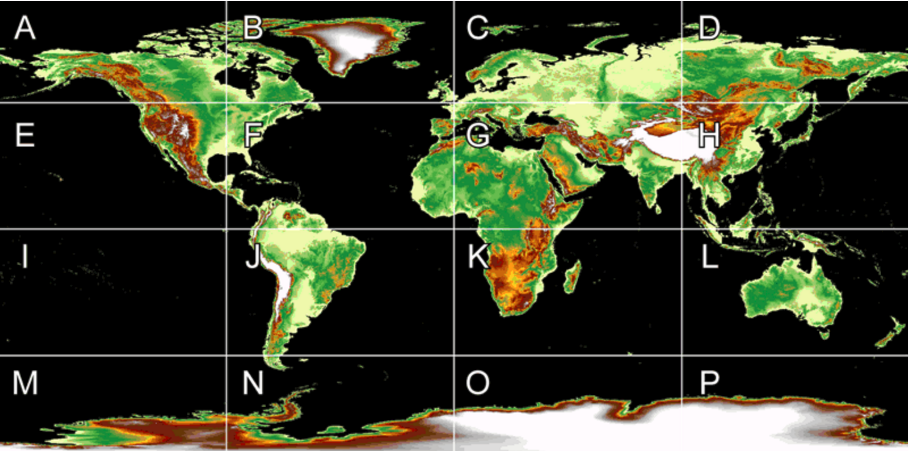
Before downloading the data, here's a quick crash course about NOAA GLOBE data. First, the file is stored in a .BIN (binary) format with HDR (header) metadata file that is maintained separately. The HDR file contains basic spatial extents and dimensions of the BIN file, which dictate how any program will read in the binary as a raster. Second, there's quite a bit of data, so scientists have cut up the DEM into 16 tiles. As seen below, the lower 48 states + Hawaii are contained in tiles "E" and "F".
To streamline our workflow, we'll write two functions: (1) one to download and read the HDR attributes, (2) one to download the BIN file and read in as a raster using the HDR attributes. As the files are not prohibitively large, we'll perform the ingest and processing in-memory.
Part 2.1: HDR Download
Nice and simply, we've written a function to download the HDR code and read it into a table as tab-separated values. The function accepts a character representing the tile index (e.g "e", "a"), creates a URL with the tile index, then reads the HDR file as a table. A cursory look at the output of the basic function shows that each row contains parameters that dictate the dimensions and spatial extent of the BIN file.
header <- function(tile_letter) {
  url <- paste("http://www.ngdc.noaa.gov/mgg/topo/data/source/esri/hdr/",tolower(tile_letter),"10s.hdr",sep="")
  temp = tempfile()
  download.file(url, temp, method="libcurl") ##download the URL taret to the temp file
  return(read.table(temp, quote="\"", stringsAsFactors=FALSE))
}

#Run function
header("e")
## V1 V2
## 1 BYTEORDER I
## 2 LAYOUT BIL
## 3 NROWS 6000
## 4 NCOLS 10800
## 5 NBANDS 1
## 6 NBITS 8
## 7 BANDROWBYTES 10800
## 8 TOTALROWBYTES 10800
## 9 BANDGAPBYTES 0
## 10 NODATA 0
## 11 ULXMAP -179.995833333333
## 12 ULYMAP 49.995833333333
## 13 XDIM 0.008333333333
## 14 YDIM 0.008333333333
## 15 FILE e10s.hdrPart 2.2: BIN Download
Reading in the DEM file involves a slight bit more effort. The function accepts the tile index and the header function produced hdr file. Using those arguments, five steps are taken:
- Download the DEM tile
- Extract spatial dimensions of the raster from the HDR file
- Create a blank raster
- Read in the DEM's binary values
- Set the binary values to the blank raster
dem_tile <- function(tile_letter,hdr_file) {

  #Load in raster package
    require(raster)

  #Download
    letter <- tolower(tile_letter)
    url <- paste("http://www.ngdc.noaa.gov/mgg/topo/DATATILES/elev/",letter,"10g.zip",sep="")
    temp = tempfile()
    download.file(url, temp, method="libcurl") ##download the URL target to the temp file
    unzip(temp,exdir=getwd()) ##unzip that file

  #Define raster file dimensions and extent from HDR file
    hdr_file[,2] <-as.numeric(hdr_file[,2])
    col= hdr_file[4,2]
    row = hdr_file[3,2]
    mat= col*row
    xmin = hdr_file[11,2]
    xmax = xmin + hdr_file[13,2]*col
    ymin = hdr_file[12,2]
    ymax = ymin + hdr_file[14,2]*row

  #Create a blank raster with certain dimensions
    bil <- raster(ncols=col, nrows= row, xmn=xmin, xmx=xmax, ymn=ymin, ymx=ymax )

  #Read in BIN file
    bin <- readBin(paste(letter,"10g",sep=""), what="integer", n=mat,endian="little", signed=TRUE, size=2)

  #Return a file tht sets BIN values into the blank raster file
    return(setValues(bil, bin))
}
How does this work when we put it together? Well, let's take tile "E" for the US West Coast/Pacific. We'll plot the result of the dem_file. Note that Rockies are clearly colored at the right of the map? This is just the beginning.
#Read in Tile "E"
  hdr <- header("e")
  dem_result <- dem_tile("e",hdr)

#Plot Tile "E"
  plot(dem_result)
Processing and Visualization
Now that we have this basic set of functions to bring in the data, we can easily pull together and merge tiles "E" and "F" and map the merged raster.
#Read in the tiles
  letters <- c("e","f")

  for(k in letters){
    hdr <- header(k)
    dem_result <- dem_tile(k, hdr)
    assign(paste("dem_",k,sep=""),dem_result)
    rm(dem_result)
    print(paste(k," - Done"))
  }
## [1] "e - Done"
## [1] "f - Done"#Merge east coast and west coast
region <- merge(dem_e, dem_f)
dim(region)## [1] 6000 21600 1#Map it!
plot(region)
Note that the raster dimension is about 129.6 million cells (6000 x 21600). That may be quite a bit more than what an interactive 3D model can handle. To process it down, we'll convert the raster into sparse matrix format, averaging every 25 cells – or just 200,000+ cells at 25-km resolution as opposed to the original 1-km resolution. In matrix form, the DEM will be backwards along the X-axis, which means we will need to flip the order of columns.
In is important to note that the different applications of DEMs require different raster resolution. NOAA's DEMs are useful at a macro scale, looking at environmental and regional issues. For small area topography, it is often useful to check for LiDAR-based data for high precision, high resolution topography.
  #Average every 25 rasters cells
    a <- aggregate(region, fact=25, fun=mean)
    a <- as.matrix(a)
    a[a < 0]<-NA

  #Flip order of columns
    a<-a[,seq(dim(a)[2],1,-1)]
    dim(a)
## [1] 240 864Now that the data is in the right form, we can use a convenient plotly package to create a 3D rendering of the US, as seen in the intro section. Of course, topography is a major determinant of how the Brazos River flows, but other datasets that contain groundtruthed water flow (e.g. USGS National Water Information Service) and vegetation data (e.g. NDVI from NASA and NOAA satellites) play large roles in the creation of environmental data services.
  #Parameter for view of 3d surface
    scene = list(
      #set where the camera will point from
        camera = list( eye = list(x = 0, y = 1, z = 1)),
      #set the canvas space proportions
        aspectratio =  list(x = 2, y = 1, z = 0.2)
        )

  #Plot map
      plot_ly(z = a, type = "surface", colors = terrain.colors(10)) %>%
        layout(scene=scene)